"Whenever a large sample of chaotic elements are taken in hand … an unsuspected and most beautiful form of regularity proves to have been latent all along."
--- Francis Galton, 19th century
We saw in Exercise 3.3 that bell shaped curves arise when we repeat rolls of dice and look at, say, the fraction of sevens. Other examples of where such curves commonly arise include:
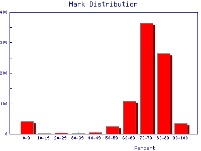
| Grade distributions for a class. This example is the Fall marks from a first year Physics laboratory at the University of Toronto. The "sample size" is 845 students. The small excess for very low marks is probably from students who have dropped the laboratory but still appear in the mark database. | |
| Heights of people. This is data for 928 people born of 205 pairs of parents. The data were taken in England by Galton in 1886. | |
| Radioactive decay. Here are data of the number counts in one second from a Cesium-37 radioactive source. The measurements were repeated 100 times. | |
Data that are shaped like this are often called normal distributions. The most common mathematical formula used to describe them is called a Gaussian, although it was discovered 100 years before Gauss by de Moivre. The formula is:
which looks like:
The symbol A is called the maximum amplitude.
The symbol
![]() is called the mean or average.
is called the mean or average.
The symbol
![]() is called the standard deviation of
the distribution. Statisticians often call the square of the standard
deviation,
is called the standard deviation of
the distribution. Statisticians often call the square of the standard
deviation,
![]() 2, the variance; we will
not use that name. Note that
2, the variance; we will
not use that name. Note that
![]() is a measure of the width of the curve: a
larger
is a measure of the width of the curve: a
larger
![]() means a wider curve. (
means a wider curve. (![]() is the lower case Greek letter
sigma.)
is the lower case Greek letter
sigma.)
The value of N(x) when x =
![]() +
+
![]() or
or
![]() -
-
![]() is about 0.6065 ×
A, as you can easily show.
is about 0.6065 ×
A, as you can easily show.
Soon it will be important to note that 68% of the area under the curve of a Gaussian lies between the mean minus the standard deviation and the mean plus the standard deviation. Similarly, 95% of the curve is between the mean minus twice the standard deviation and the mean plus twice the standard deviation.
In the quotation at the beginning of this section, Galton refers to chaotic elements. In 1874 Galton invented a device to illustrate the meaning of "chaotic." It is called a quincunx and allows a bead to drop through an array of pins stuck in a board. The pins are equally spaced in a number of rows and when the bead hits a pin it is equally likely to fall to the left or the right. It then lands on a pin in the next row where the process is repeated. After passing through all rows it is collected in a slot at the bottom. After a large number of beads have dropped, the distribution is Gaussian.
A simulation of a quincunx is available here.
Question 4.1. In Exercise 3.3 you were asked to find a numerical way of measuring the width of the distributions. One commonly used method is to find the "full width at half the maximum" (FWHM). To find this you determine where the number of data is one-half of the value of the maximum, i.e. where N(x) = A/2. There will be two such points for a bell shaped curve. Then the FWHM is the difference between the right hand side value and the left hand side value of x. For a Gaussian distribution what is the mathematical relationship between the FWHM and the standard deviation?
Question 4.2. You have a large dataset that is normally distributed. If you choose one data point at random from the dataset, what is the probability that it will lie within one standard deviation of the mean?
|
In everyday usage the word chaotic, which has been used above, means utter confusion and disorder. In the past 40 years, a somewhat different meaning to the word has been formed in the sciences. Just for interest, you may learn more about scientifically chaotic systems here. A difference in the meaning of words in everyday versus scientific contexts is common; examples include energy and momentum. |
![]()
![]()
This document is Copyright © 2001, 2004 David M. Harrison
 |
This work is licensed under a Creative Commons License. |
This is $Revision: 1.6 $, $Date: 2004/07/18 16:40:00 $ (year/month/day) UTC.